nanogpt

I trained a 124M parameter language model from scratch on a single A100 GPU in about an hour. That’s it.

Here’s what it generates:

prompt: What is the answer to life, the universe, and everything?
generated_text: The answer is yes. What can I do for my life, my family or even a little piece of me with all that I have lost in this time? How could I have changed that and made it work again on my own? How could I have made some changes to my life over the years so that it has been taken into account when it comes back from this loss? How could I make myself more productive? In addition, what would be my priority if I had no other words to say to me now? Would I choose to follow up any of these things and give up? What would happen if someone else was involved in my

I started with Andrej Karpathy’s Let’s reproduce GPT-2 (124M), then the modded-nanogpt speedrun to make training as fast as possible.

Baseline

I started simple. Plain PyTorch, no tricks. Just the standard GPT-2 architecture so I have something that works before making it fast.

Model

config:

@dataclass
class GPTConfig:
    vocab_size: int = 50257
    context_length: int = 1024
    n_embed: int = 768
    num_layers: int = 12
    n_head: int = 12

Architecture:

• Token embeddings + position embeddings (learned)
• 12 transformer blocks (attention + MLP)
• Pre-norm (LayerNorm before attention/MLP)
• Residual connections
• GELU activation

class GPT(nn.Module):
    def __init__(self, config):
        super().__init__()
        self.transformer = nn.ModuleDict(dict(
            wte = nn.Embedding(config.vocab_size, config.n_embed),
            wpe = nn.Embedding(config.context_length, config.n_embed),
            h = nn.ModuleList([Block(config) for _ in range(config.num_layers)]),
            ln_f = nn.LayerNorm(config.n_embed)
        ))
        self.lm_head = nn.Linear(config.n_embed, config.vocab_size, bias=False)
        # Weight sharing: saves ~40M parameters
        self.transformer.wte.weight = self.lm_head.weight

Weight initialization

def _init_weights(self, module):
    if isinstance(module, nn.Linear):
        torch.nn.init.normal_(module.weight, mean=0.0, std=0.02)
        if module.bias is not None:
            torch.nn.init.zeros_(module.bias)
    if isinstance(module, nn.Embedding):
        torch.nn.init.normal_(module.weight, mean=0.0, std=0.02)

I use std=0.02. GPT-2 paper used this. It is close to Xavier scaling 1/√768 ≈ 0.036 but 0.02 works fine. I also scale the attention output projection by 1/√(2 * num_layers) to keep the residual stream stable. Without this, deep networks explode.

Data

Dataset: FineWeb 10B (sample-10BT)

• Development: 20M-token subset
• Full training later: 10B

Tokenizer: GPT-2 BPE (tiktoken).

Loader:

class TokenDataLoader:
    def __init__(self, data_root, B, T):
        self.B = B
        self.T = T
        self.shards = sorted([...])
    
    def next_batch(self):
        buf = self.tokens[self.current_position : self.current_position + needed]
        x = buf[:-1].view(B, T)  
        y = buf[1:].view(B, T)    
        return x, y

Training Setup

Hyperparameters:

total_batch_size = 524288       
batch_size = 32               
sequence_length = 1024        
grad_accum_steps = 16         
learning_rate = 3e-4      

Training loop:

for step in range(max_steps):
    optimizer.zero_grad()
    loss_accum = 0.0
    for micro_step in range(grad_accum_steps):
        x, y = train_loader.next_batch()
        x, y = x.to(device), y.to(device)   
        _, loss = model(x, y)
        loss = loss / grad_accum_steps 
        loss_accum += loss.detach()
        loss.backward()
    optimizer.step()

So here is our starting point: it took 20 minutes to process 20M tokens on an A100 GPU. We hit 16,700 tokens/sec with a final loss of 7.04. The code works, but it’s so slow. Let’s make it faster. Check the log

Making training fast

The math is correct, but it takes too long. PyTorch has a few built-in tricks to make the GPU work smarter.

Mixed precision

Deep learning uses 32-bit floats by default. That is extremely precise, but tensor cores, the specialized math engines inside the A100 are built to smash through 16-bit numbers way faster.

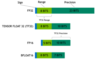
TensorFloat-32 (TF32): TF32 is a cheat code. It keeps the giant range of 32-bit numbers but trims the decimal precision to 10 bits. The tensor cores love it. One line turns it on:

torch.set_float32_matmul_precision('high')

True mixed precision: For an even bigger jump, we force the heavy lifting like massive matrix multiplications into true 16-bit mode. PyTorch’s torch.autocast handles the traffic automatically: safe math stays 32-bit, heavy math drops to 16-bit.

You have two choices here: Float16 or Bfloat16.

Float16 is fast and runs anywhere, but it has a tiny numeric range. Tiny gradients can underflow to plain zero, completely breaking the learning process. To fix that, you use a GradScaler to scale up the loss going backward, then shrink it back down before the optimizer steps.

Float16 recipe:

scaler = torch.cuda.amp.GradScaler() 
with torch.autocast(device_type='cuda', dtype=torch.float16):
    _, loss = model(x, y)
    loss = loss / grad_accum_steps

scaler.scale(loss).backward() # Scale gradients
scaler.step(optimizer)        # Unscale & Step
scaler.update()               # Update scale factor

Bfloat16 is the newer, better option if you have modern hardware. It keeps the huge range of FP32 by trading off precision bits. Gradients survive just fine. No scaler needed. It’s clean and simple.

Bfloat16 recipe:

with torch.autocast(device_type='cuda', dtype=torch.bfloat16):
    _, loss = model(x, y)
    loss = loss / grad_accum_steps
    loss_accum += loss.detach()

# Backward pass (Simple! No scaler needed)
loss.backward()

I used bfloat16 autocast combined with TF32 for maximum speed.

torch.compile

It’s a magic line that makes everything faster.

model = torch.compile(model, dynamic=True)

Normally, PyTorch is eager. It fires one GPU kernel per operation. The GPU has to load data from its big, slow memory (HBM), run the math, and write it back. Every single time.

torch.compile() does two huge things:

1. Kernel fusion: It squashes multiple operations into one single kernel. The data stays in the on-chip SRAM instead of doing endless round-trips to HBM.
2. Graph optimization: It drops redundant code, reorders math for better speed, and picks exactly the right CUDA kernels for the hardware.

Why dynamic=True? PyTorch typically compiles kernels expecting exact, fixed tensor shapes. If your input dimensions vary even slightly, the compiler halts training for a CPU recompilation. The dynamic=True flag forces it to generate flexible kernels that gracefully handle varying dimensions.

The first run takes 1–2 minutes to build these custom kernels. After that, the training steps just fly. If you want a deep dive into this compilation magic, the official PyTorch compiler tutorial is an excellent resource.

Flash Attention

Self-attention is mathematically simple: just two matrix multiplies (Q @ K^T, then @ V) and a softmax. But the memory round trips are what kills performance. Here is what happens in baseline code:

1. You compute Q @ K^T and write that N×N matrix to the GPU’s slow main memory (HBM).
2. You read it back from HBM to apply softmax, then write the new N×N probabilities back to HBM.
3. You read it from HBM one last time to multiply it by the V matrix.

During the backward step, the nightmare repeats. You either store that giant matrix in HBM the whole time, or you discard it and recompute it from scratch which means doing all those slow HBM matrix trips again. The end result? Your blazing fast tensor cores sit completely idle, just waiting for data to arrive.

The bottleneck isn’t the math. It’s the memory bandwidth.

Flash Attention fixes this with one core idea: stay in SRAM.

It chops the massive matrices into tiny blocks that fit completely inside the ultra-fast on-chip SRAM. Then it fuses the entire attention block into one smart, highly optimized kernel:

1. Move a tiny block from slow HBM to fast SRAM.
2. Multiply it.
3. Normalize it on the fly.
4. Multiply by the V block.
5. Write only the final, small output back to HBM.

That’s it. The massive attention matrix never even materializes in slow memory. During backprop, it recomputes everything block-by-block entirely in SRAM. The extra math required to recompute is practically free compared to the massive cost of reading from HBM.

PyTorch ≥ 2.0 has it built-in. It’s literally one line:

attn_output = F.scaled_dot_product_attention(q, k, v, attn_mask=None, dropout_p=0.0, is_causal=True)

The Results. Just by adding these tricks, the exact same model running on the exact same 20M tokens on an A100 zoomed to an incredible 200,000 tokens/sec! 😅 The training time dropped from a slow 20 minutes down to just 2.66 minutes. The loss stayed completely stable at 7.03. Same hardware, same math, just a huge speedup. Check the log

Architectural Changes

Kernel and compiler tricks broke the memory bottlenecks, but the math under the hood is still standard 2019-era GPT-2. We can swap out a few archaic components for modern, leaner alternatives that are faster and train better.

Rotary Positional Embeddings

So far, the model implicitly encoded position like the original GPT-2: it learned a giant 1024x768 lookup table for the token positions, fetching one vector per index and adding it directly to the token embedding.

wpe = nn.Embedding(config.context_length, config.n_embed)

This works, but it’s fundamentally flawed. The model just memorizes absolute positions as arbitrary vectors. It doesn’t inherently understand that the distance between tokens at index 5 and 6 is exactly the same as the distance between 505 and 506. We want the attention mechanism to natively grasp relative distance.

Rotary Positional Embeddings (RoPE). Instead of blindly adding a learned position vector, we rotate the Query and Key vectors inside the attention matrix by an angle that corresponds to their position.

If you want a brilliant, intuitive deep-dive into this math, I highly recommend watching Zachary Huang’s Give me 30 min, I will make RoPE click forever video.

RMSNorm

The standard GPT-2 uses PyTorch’s LayerNorm. LayerNorm computes the mean, subtracts it to center the values, and then applies a learned scale and bias.

I replaced it with RMSNorm (Root Mean Square Normalization). RMSNorm completely drops the mean-centering operation and the learned bias term. By just scaling the weights, RMSNorm strips out unnecessary operations and significantly simplifies the computation. It preserves model performance while being computationally cheaper.

def norm(x: torch.Tensor):
    return F.rms_norm(x, (x.size(-1),))

Squared ReLU

I also swapped out the standard GELU activation function inside the MLP for Squared ReLU (ReLU²).

GELU is mathematically squishy. It relies on tanh and expensive exponential functions under the hood to smooth out its curve, which are slow to evaluate. ReLU² is literally just max(0, x)^2.

Vocabulary Padding

The official GPT-2 tokenizer vocabulary size is 50,257.

This is a nightmare for GPUs. Tensor Cores are specifically built around powers of two. When your embedding matrix dimensions aren’t clean, even multiples, the GPU suffers from memory misalignment and wasted cycles.

So, I padded the vocabulary size to 50,304 (50,257 + 47). This small change ensures that all of our embedding and lm-head linear layer tensor dimensions are nice round numbers. It’s a tiny change that keeps the Tensor Cores happy.

The Results. Adding these modern architectural tweaks to our baseline 20M-token slice pushed our throughput up to 205,000 tokens/sec. The model finished its training run in an astonishingly fast 1.82 minutes, and the final loss dropped to 6.93. Check the log

Going All In

The first three sections were just experiments on 20M tokens. The next goal: a 5 billion token pretraining run. The target is to hit around val_loss ≤ 3.28 on FineWeb-10B in about two hours on a single A100.

To hit this target, I made some upgrades in three areas: the model architecture, the data loader, and the optimizer.

Model Upgrades

QK-Norm. At aggressive learning rates, the Query and Key norms can explode. Their dot products blow up, NaNs appear, and the run dies.

To fix this, I applied RMSNorm to the Queries and Keys right after their linear projections (before RoPE).

q = F.rms_norm(q, (H,))
k = F.rms_norm(k, (H,))

These two lines are what allowed me to run the Muon optimizer with a learning rate of 0.02 without instability.

U-Net Skips. Vanilla transformer layers only see out to the layer directly below them. Taking inspiration from U-Nets, I split the stack. Layers 1-6 stash their residuals in a list. Layers 7-12 pop those residuals off and add skips from their symmetrically mirrored shallow layer (Layer 7 pulls from 6, Layer 8 pulls from 5, up to Layer 12 pulls from 1).

skips = []
for i, block in enumerate(self.blocks):
    if i < self.half_n:  
        skips.append(x)
    else:        
        x = x + skips.pop()
    x = block(x, cu_seqlens, pos, max_seqlen)

Shallow signals (like fundamental syntax and frequency patterns) reach deep into the network without going through twelve sequential transforms.

Logit Soft-Capping. High entropy is good, but unbounded logits can let a single class dominate the softmax distribution. The model collapses, entropy vanishes, and it stops learning the long tail of the vocabulary.

Logit soft-capping, popularized by Gemma 2 and the modded-nanogpt is essentially a smooth, differentiable version of clipping. Instead of a hard cut-off, it uses a scaled tanh to gently squash logits into a fixed range (usually ±30):

logits = self.config.logit_softcap * torch.tanh(logits / self.config.logit_softcap)

Training System Upgrades

Document Packing. The basic data loader blindly cuts one long stream of text into chunks. This is bad because the model ends up reading half of one document and half of a completely unrelated document in the same sequence.

The easy fix is to just pack your documents perfectly back-to-back, separating them with a <|endoftext|> token and give it to the model as a single long sequence. But how do you prevent the model from looking across those packed boundaries?

The easiest way to handle this is by using FlashAttention library’s varlen function. You simply give it a list of your document lengths (cu_seqlens). It automatically resets the attention mask at every boundary, guaranteeing the model never reads across different documents. No complicated custom masking required:

y = flash_attn_varlen_func(
    q, k, v,
    cu_seqlens_q=cu_seqlens, cu_seqlens_k=cu_seqlens,
    max_seqlen_q=max_seqlen, max_seqlen_k=max_seqlen,
    dropout_p=0.0, causal=True,
)

Muon Optimizer. AdamW is the standard default, but we can do a lot better.

Muon (Momentum Orthogonalized by Newton–Schulz) is a specialized, incredibly efficient optimizer designed specifically for the NanoGPT speedrun by Jordan et al.

I highly recommend reading the original Muon blog post for the deep mathematical details.

Because Muon relies on specific 2D matrix properties of internal linear layers, it isn’t a drop-in replacement for everything. We simply split the workload: Muon optimizes the massive hidden transformer blocks, while standard AdamW handles the token embeddings and the language model head.

muon_optimizer = Muon(model.blocks.parameters(), lr=0.02, weight_decay=0.01)
adam_optimizer = torch.optim.AdamW(
    model.wte.parameters(), lr=0.006, betas=(0.9, 0.95), weight_decay=0.1, fused=True,
)

Learning-Rate Schedule. I used a simple trapezoidal schedule. It has three easy phases: a fast warmup, a long flat hold at maximum speed, and a gentle cooldown.

Moment of Truth

With all of the above combined, I hit go and let the A100 run through 1,500 steps. The loss started at 11.0 and dropped fast, below 5.0 by step 125, below 4.0 by step 400. By the end, the training loss bottomed out at 3.41 with a best validation loss of 3.46.

The whole run took 69 minutes. The model processed 786 million tokens at an average of 191,000 tokens/sec, with 35.8% MFU across the entire run.

Logs: WandB run · Raw log: nanogpt-1500.txt

Training speed is great, but does it actually generate coherent text? To find out, I ran a benchmark comparing nanogpt head-to-head against the official OpenAI GPT-2 model on the WikiText-2 dataset.

nanogpt hit a perplexity of 56.47, while the official GPT-2 sits at 27.22. Even with all the architectural upgrades I added (RoPE, RMSNorm, U-Net skips, and Squared ReLU), nanogpt only read 786 million tokens. OpenAI trained GPT-2 on roughly 40 billion tokens, 50x more text! A powerful architecture accelerates learning, but the model needs to read more data to get smarter.

The next step: let the GPU cook for longer. Training for 3,000 steps so the model can go through more of the FineWeb-10B dataset. Let’s see how close to that OpenAI baseline we can get.

Resources

The architecture and training recipe are heavily inspired by Keller Jordan’s modded-nanogpt speedrun and Tyler Romero’s contributions. The Muon optimizer originates from this work. And of course, the whole thing stands on the shoulders of Andrej Karpathy’s nanoGPT and minGPT, which showed that a GPT implementation doesn’t need to be 10,000 lines.